Learning Heuristics for the TSP by Policy Gradient 논문 리뷰 및 설명

Learning Heuristics for the TSP by Policy Gradient

이전의 NCO를 읽고 오시면 도움이 됩니다.

Abstract

• 이 논문은 Combinatorial Optimization Problem을 해결하는데 ML이 heuristic algorithm과 결합하여 좋은 성능을 낼 수 있음을 보입니다. 이 때, encoder와 decoder 모두 LSTM을 제거한 점이 눈에 띕니다.

Introduction

Reinforcement Learning Perspective for the TSP

Neural Architecture for TSP

• TSP 문제는 n개의 도시 s에서 모든 도시 n개를 방문하여 제자리로 돌아오는 최단거리를 찾는 문제입니다. 이 때 cost는 전체 edge의 weights이고, stochastic policy \(p_\theta(\pi\vert s)\)는 neural network와 policy gradient를 통해 이를 배우게 됩니다.
• 논문의 구조는 기존의 encoder decoder 구조를 사용합니다. encoder는 input set \(I = (i_1,...,i_n)\)에 대해 representation \(Z = (z_1,...,z_n)\)로 mapping하고, \(Z\)에 대해 decoder는 순차적으로 output \(O = (o_1,...,o_n)\)을 생성해냅니다. 이때 이 과정은 자신의 output이 다시 input으로 들어와 자기회귀된다는 의미의 “Auto-Regressive하다”라는 표현을 합니다.

TSP Setting and Input Preprocessing

• 논문은 2D Euclidean TSP에 집중합니다. 이 때 Principal Component Analysis(PCA)를 통해 input이 회전에 대해 invariance하도록 만들어 사용합니다.

Encoder

• encoder는 각 city에 대한 representation을 만드는 과정인데, 기존 연구와 다르게 LSTM을 사용하지 않고, multi-head-attention을 사용합니다. 좀 더 구조를 자세히 살펴보자면 다음과 같습니다.

• TSP encoder

  

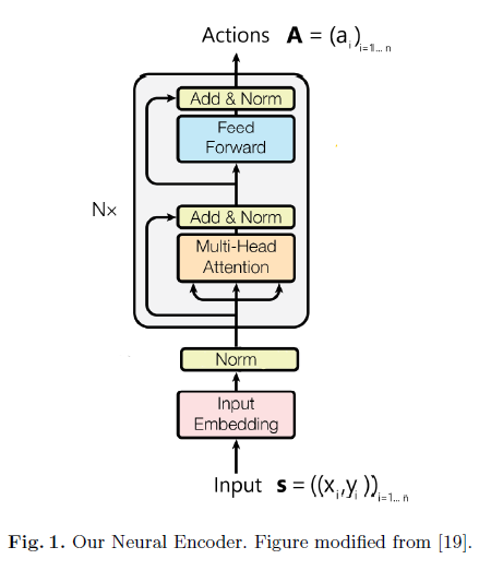
• 그림과 같이 input은 embedding되고, batch norm이 적용된 cities를 받습니다. 그 다음 Multi-head attention과 Feed-Forward로 이루어진 layer를 N번 거치게 됩니다.
• Multi-Head Attention

  • 각 city의 latent는 key query value가 되어 trainable weights를 통해 linear transformation된 후 ReLU로 non-linearity를 더해 다음과 같은 연산을 진행합니다.

    \[Attention(Q;K;V) = softmax(\frac{QK^T}{\sqrt{d}})V\]

    이 연산을 통해 각 city는 새로운 representation을 얻게되며, 이 때 기존 transformer의 논문처럼 multi head를 사용하기 때문에 자세히는 h개로 쪼개어 head에 들어가 계산된후 합쳐져 원래 dimension을 유지하게 됩니다.

• Feed-Forward
  • 두개의 position-wise linear transformation(1d convolution)와 ReLU로 이루어져있는데, 요즘 transformer에선 fc로도 많이 처리를 합니다.

Decoder

• 기존의 decoder는 다음과 같은 수식으로 나타낼 수 있습니다.

  \[p_\theta(\pi \vert s) = \prod^n_{t=1}p_\theta(\pi(t) \vert \pi(<t),s)\]

  이를 해결하기 위해서 기존에 LSTM decoder를 사용했지만, 여기서는 이전의 3개의 action만을 input으로 넣어줘도 잘 동작함을 확인하였고 LSTM을 제거했습니다. 그러므로 다음 action을 위한 query는 다음과 같이 나타낼 수 있습니다.

  \[q_t = ReLU(W_1a_{\pi(t-1)} + W_2a_{\pi(t-2)} + W_3a_{\pi(t-3)}) \in \mathbb{R}^{d'}\]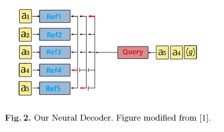

  

• Pointing Mechanism

  • Pointing은 기존의 방법과 같은데, cities \(A = (a_1,...,a_n)\)와 query를 이용하여 pointing을 진행하게 됩니다. 이 때, NCO에서 제시했던 clipping과 temperature를 넣는 모습을 볼 수 있습니다.

    \[\forall{i} \leq n, u^t_i = \left\{\begin{matrix}v^Ttanh(W_{ref}a_i +W_qq_t)\ \ if \ i \notin \{\pi(0),..., \pi(t-1)\}\\ - \infty \ \ \mathrm{otherwise}\end{matrix}\right.\] \[p_\theta(\pi(t)\vert \pi(<t)) = softmax(C tanh(u^t/T))\]

Training the Model

• Policy Gradient and REINFORCE

  • objective는 다음과 같이 나타낼 수 있습니다.

    \[\min J(\theta \vert s ) =\mathbb{E}_{\pi \sim p_\theta(\cdot \vert s)}[r(\pi \vert s )]\]

    graphs는 training set의 분포 \(S\)로 부터 추출되므로 이는 다음과 같이 나타낼 수 있습니다.

    \[\min J(\theta) =\mathbb{E}_{s \sim S}[r(\pi \vert s )]\]

    이를 REINFORCE trick을 사용한 뒤 critic network에 의한 baseline을 도입하면 다음과 같이 나타낼 수 있습니다.

    \[\nabla _{\theta} J(\theta \vert s ) = \mathbb{E}_{\pi \sim p_\theta(\cdot \vert s)}[(r(\pi \vert s ) -b_\phi(s))\nabla _\theta\log{(p_\theta(\pi \vert s))}\]

    이를 Monte-Carlo sampling을 통해 근사하여 나타낼 수 있습니다.

    \[\nabla _{\theta} J(\theta \vert s ) = \frac{1}{B}\sum^B_{k=1}[(r(\pi_k\vert s_k ) -b_\phi(s_k))\nabla _\theta\log{(p_\theta(\pi_k \vert s_k))}\]

    이를 통해 Stochastic Gradient Descent와 함께 policy parameter \(\theta\)를 update하게 됩니다.

• Critic

  • critic은 actor와 같은 encoder를 사용하며, query \(q\)에 zero vector를 넣어 pointing distribution \(p_\phi(s)\)를 만듭니다. 이를 통해 NCO처럼 glimpse vector를 만드는데, 이는 전체 city에 대한 weighted sum을 통해 baseline에 영향을 주는 cities에 대한 가중치합을 만드는 것과 같다고 설명했었습니다. 이는 수식으로 나타내면 다음과 같습니다.

    \[gl_s = \sum^n_{i=1}p_\phi(s)_ia_i\]

    이후 두개의 fc를 거쳐 scalar 값이 나오게 됩니다. critic은 reward와의 MSE를 통해 학습됩니다.

References

• Learning Heuristics for the TSP by Policy Gradient

치명적인 단점으로 fixed length input, input이 크고 서로간의 적은 상관성을 가진 경우에 대해 과도한 연산을 하게됩니다.